Issue, No.31 (September 2024)

Socio-demographic Changes and Income Inequality^*

by Ella-Marie Assal, (University of Antwerp)

In recent decades, income inequality has been on the rise in many European countries. One potential driver of this trend could be structural changes in the socio-demographic composition of these countries. Many nations have experienced an aging population, significant changes in household formation, and higher levels of educational attainment. In this note, we explore how these socio-demographic changes have impacted income inequality in six continental European countries over a thirty-year period, from 1990 to 2021.

Methodology

We use the LIS data for Austria, Belgium, France, Germany, Luxemburg and the Netherlands for 1990 (or closest subsequent data year) and 2021 (or the most recent available year). To evaluate the effect of changes in socio-demographic characteristics on the income distribution, we construct counterfactual income distributions. Specifically, we compare the observed, recent income distribution in year t with a counterfactual distribution with the incomes of year t but the socio-demographic composition of a previous year t’. The difference between the actual and counterfactual income distributions then represents the effect of the changes in socio-demographic characteristics.

The counterfactual income distribution is estimated using the semi-parametric reweighting technique as introduced by DiNardo et al. (1996).

Let ƒ_t (γ) be the income distribution at date t:

Where ƒ(y|z,t_y=t) is the distribution of income y conditional on socio-demographic variables z at date t, and ƒ(z,t_z=t) is the distribution of demographic variables at date z. It is possible to formulate a counterfactual income distribution ƒ_C(γ):

Where ƒ(z,t_z=t’) is now the distribution of demographic variables at date t’. The counterfactual income distribution can be obtained by reweighting the conditional income distributions:

Where the reweighting function ω(z) is defined as:

Which can be rewritten using Bayes’ rule:

Conditional probabilities Pr (t_z=t’ | z) and Pr (t_z=t | z) can be easily estimated using standard techniques for binary response. We use probit models.

Note that the correct interpretation of the counterfactual is as follows: “What would the income distribution at time t have looked like had socio-demographic characteristics remained as they were at time t’, but everything else is as observed in time t?”, since the reweighting method keeps constant the income distribution conditional on these characteristics. Consequently, the counterfactual income distribution does not capture equilibrium effects of changing socio-demographic characteristics. For example, the method allows us to capture the effect of the increasing share of the population at retirement age on income inequality, but will not take into the effects of the pressure of an aging population on the incomes conditional on age. In this sense, this reweighting method is a static accounting exercise rather than a dynamic economic model.

Results

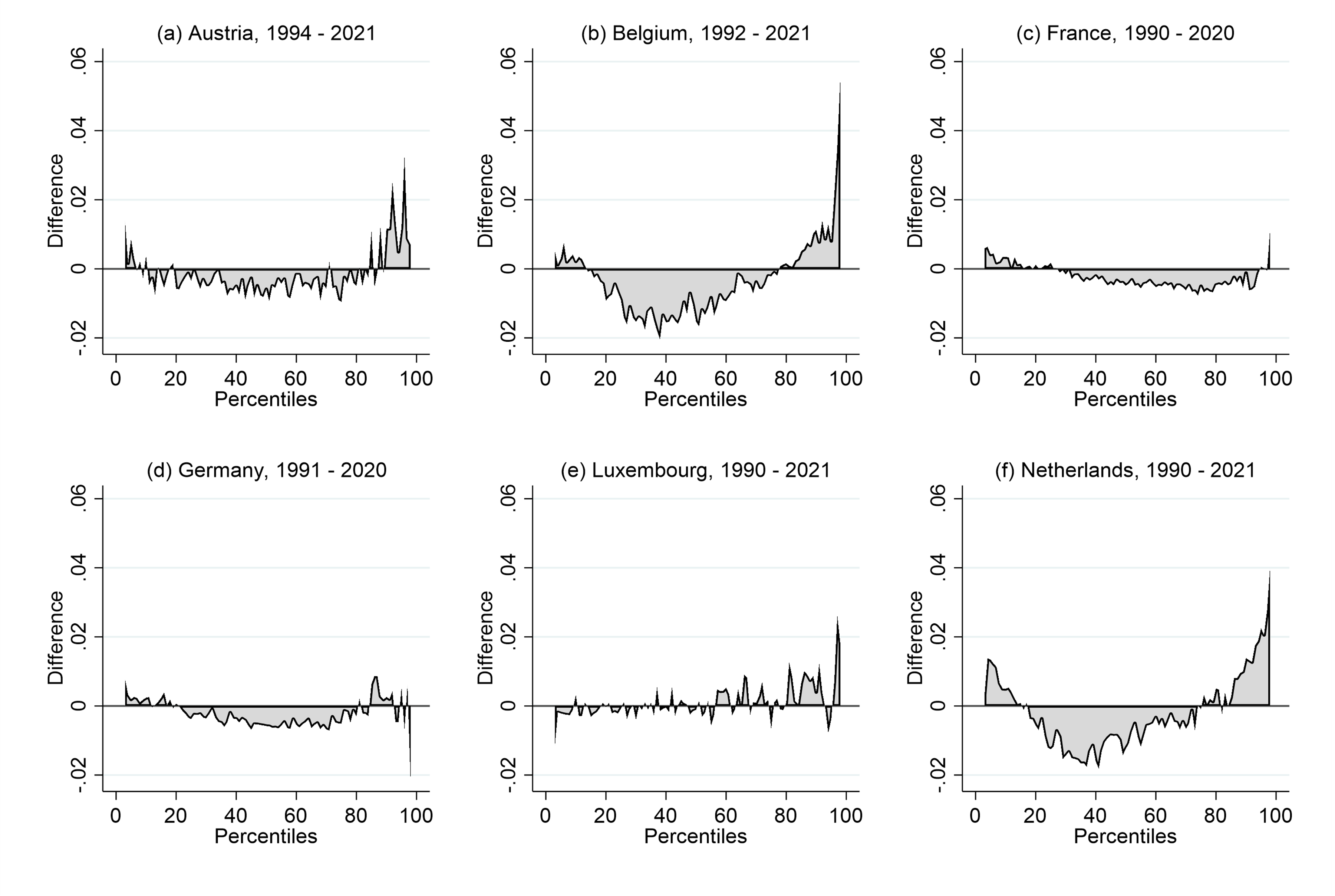
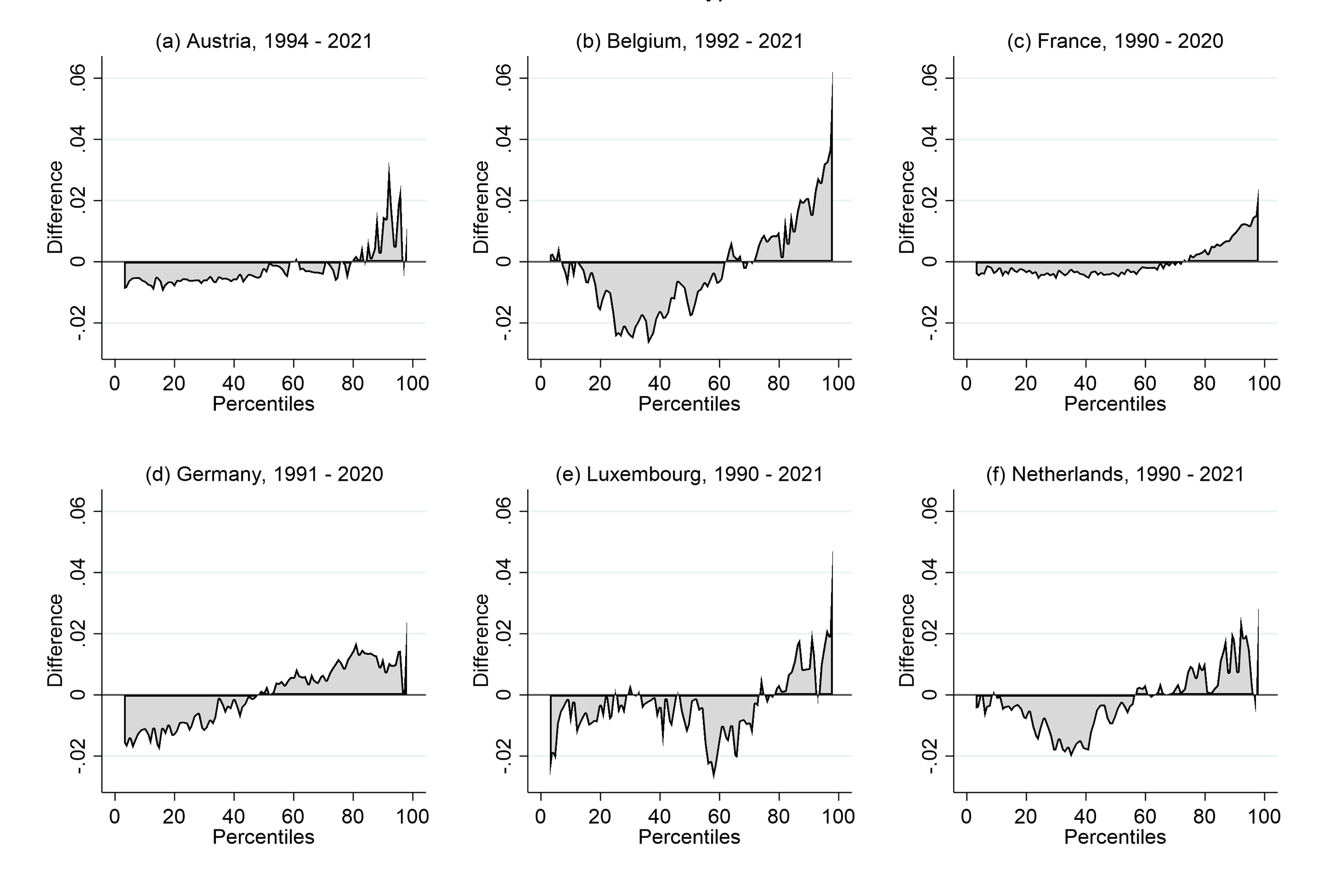
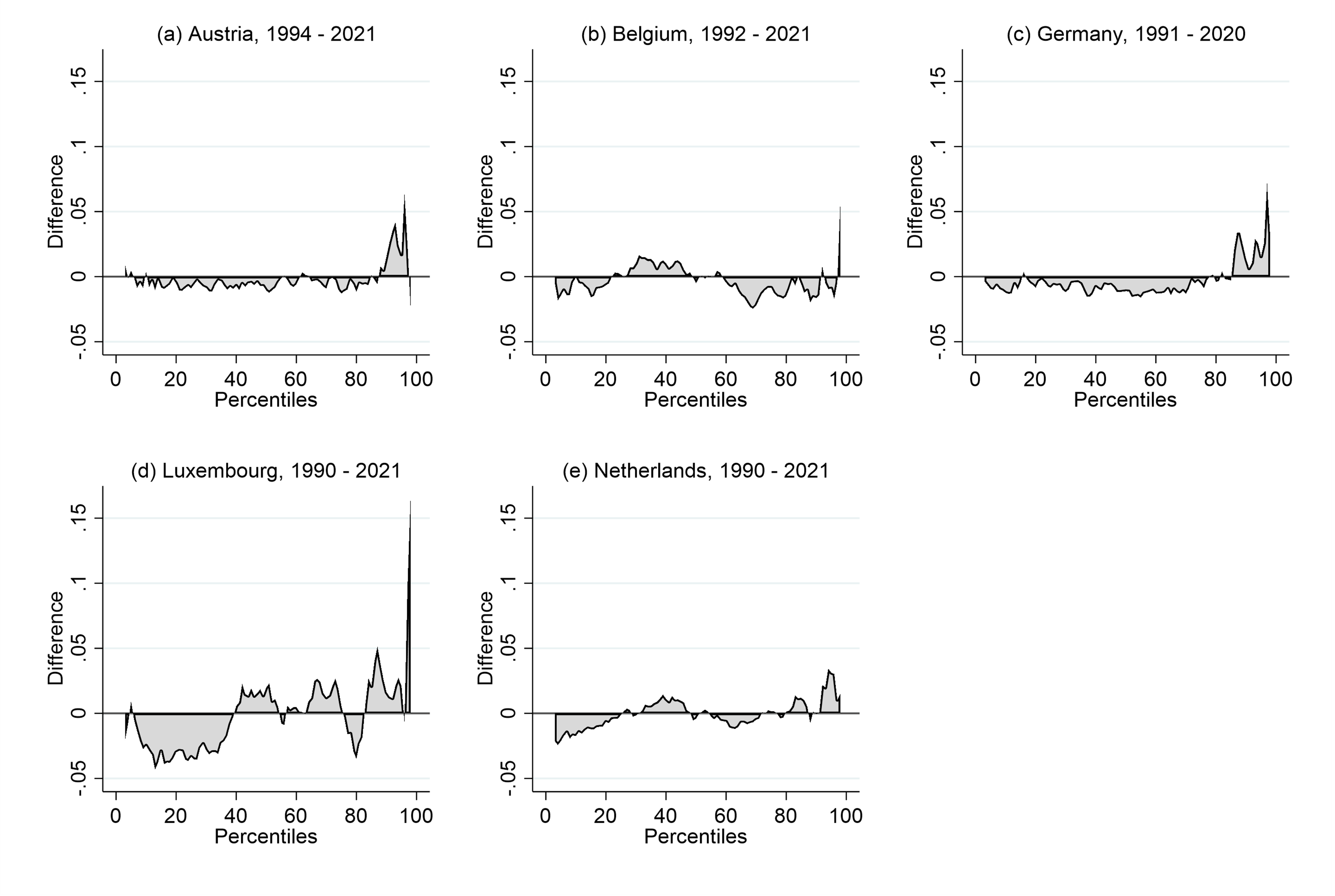
We present the effect of the socio-demographic change on the income distribution by showing the difference between the mean-normalized quintile functions (Pen’s parades) for the observed income distribution and the counterfactual income distribution. Negative values indicate that the de-meaned incomes at a certain quantile of the distribution have decreased due to the socio-demographic change, while positive values imply that the de-meaned incomes at this quantile have increased because of it. Since we are examining de-meaned quantile functions, any loss will be offset by a gain elsewhere in the distribution. In other words, the surface of the grey area in the figures below will always sum up to zero¹. Monotonically increasing or decreasing lines indicate, respectively, a clear increase or decrease in income inequality. In the following three figures, we look at the effect of population ageing, changes in household compositions and increasing educational attainments, respectively.

Figure 1: Difference between observed mean-normalized quantile function and counterfactual with reweighted age categories.

Notes:Vertical axis shows difference between the observed and counterfactual mean-normalized quintile functions. Five age categories considered for the counterfactual: under 16 years, 17-29 years, 30-49 years, 50-64 years, and 65 and over.

As in many countries, continental European welfare states have been facing the challenges of population aging. Over the past few decades, rising life expectancy and declining fertility rates have led to a substantial increase in the proportion of elderly individuals. Notably, in most of these countries, there has been not only an increase in the elderly population, who typically fall into low-income categories due to their dependence on oftentimes low pension benefits, but also an increase in the proportion of 50–64-year-olds. This last age group is usually better off compared to the rest of the population, benefiting from relatively high wages and often no longer financially burdened by dependent children.

As shown in Figure 1, the effect of the ageing population on the income distribution is generally small. The differences between the observed and counterfactual de-meaned income quantile functions are largest in Belgium and the Netherlands. Generally, the changing age distribution has come with small increases in relative incomes at the very bottom of the distribution, decreases for the majority of the distribution (from percentiles 10 to 80), and more pronounced increases at the top of the distribution. One exception is Luxemburg, which has seen quite a non-typical ageing evolution due to high migration rates. Given these patterns, where the largest gains are at the top, the figures suggest that population ageing has slightly increased income inequality.

Figure 2: Difference between observed mean-normalized quantile function and counterfactual with reweighted household types.

Notes:Vertical axis shows difference between the observed and counterfactual mean-normalized quintile functions. Five household types reweighted in the counterfactual: Single, couple with children, couple without children, single parent and a residual category.

Given overall declines in marriage rates, rising divorce rates and decreasing fertility levels, there has been a decrease of individuals living in “traditional” households – consisting of a couple with children – in all six countries analyzed. This decline is generally accompanied by an increase in the number of singles (both with and without children) and an increase in couples without children. Typically, singles, and especially single parents, are found at the lower end of the income distribution, while couples without children are often at the higher end.

Figure 2 shows that the effect of the changing household types is quite similar for all countries in the analysis. Generally, we see a near to monotonic pattern where the relative incomes for the bottom three quarters of the distribution decrease, while the relative incomes for those in the top 25% increase. This pattern is particularly pronounced in Belgium, Germany and the Netherlands. Consequently, it is evident that in all the countries analyzed, the changing household composition (i.e. the shift away from the “traditional” household) is contributing to an increase in income inequality.

Figure 3: Difference between observed mean-normalized quantile function and counterfactual with reweighted education levels.

Notes:Vertical axis shows difference between the observed and counterfactual mean-normalized quintile functions. Three education levels reweighted in the counterfactual based on highest attained education level: low (no secondary education degree), middle (secondary education degree) and high (tertiary education degree). France not included in graph because highest education level attained not available for 1990.

Finally, Figure 3 shows the effect of the increasing education levels. In all countries in the analysis, the majority of the population was low educated in the beginning of the 1990s. However, educational attainment had increased since then, causing an increased proportion of the population in the middle and highly educated categories. One might intuitively expect that when more people join the “well-off” group, inequality decreases. However, how the distribution of education levels impacts income inequality depends on the starting point. A society where the majority of the population is low educated (which was the case in the early 1990s) is likely to be more equal than one in which workers are more distributed across education levels (think of Kuznet’s curve).

Figure 3 demonstrates that the rise in educational attainment has indeed contributed to increasing inequality. In France and Germany, the effect is quite clear: there are small losses for the bottom 80 percent of the income distribution and gains for the top 20 percent. In Belgium, Luxembourg, and the Netherlands, the losses and gains are more dispersed across the distribution, but generally, there are losses at the bottom and gains at the top. The results for Luxembourg are particularly pronounced, mainly due to a more dramatic shift in educational levels driven by the increase of highly skilled labor migration.

As was the case for the previous results, keep in mind that the graphs in Figure 3 do not take into account any indirect effects. In reality, the returns to education are influenced by the distribution of the education levels in the workforce.

Conclusion and discussion

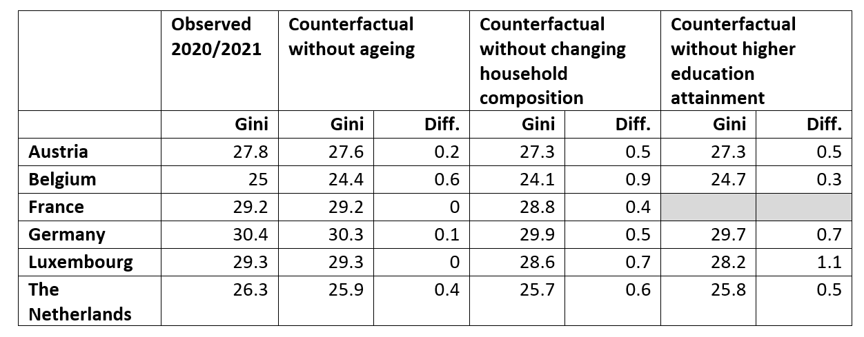
The effects of socio-demographic changes on income inequality in each country are summarized in Table 1. The analysis reveals that these changes can partly explain the upward trends in income inequality, indicating that structural socio-demographic forces are at play. The effects of aging are minimal or even negligible. However, changes in household composition have a more pronounced positive effect on inequality. Finally, while the impact of educational attainment is not always clear-cut, it also appears to contribute to increasing inequality.

It is important to note that these findings reflect only the direct effects of socio-demographic changes. Furthermore, demographic shifts are just one piece of the puzzle. These countries have also experienced significant societal changes in the labor market, tax-benefit systems, and other areas that influence income inequality. Further evaluations would be needed to fully understand the interplay of these factors and their impact on income distribution.

^* This article is an outcome of a research visit carried out in the context of the (LIS)²ER initiative which received funding from the Luxembourg Ministry of Higher Education and Research.

¹ It is possible that this is not always clearly reflected in the figures, which exclude the first and last percentile because of potential extreme values.

References